Example using PySB with ODE simulations
import matplotlib.pyplot as plt
import numpy as np

from pysb.examples.robertson import model
from pysb.simulator import ScipyOdeSimulator
from simplepso.logging import get_logger
from simplepso.pso import PSO
For this example, we are going to train the model to some made up data. Please refer to a PySB tutorial if you are new to PySB. This tutorial assumes you have knowledge of PySB.
# setup model and simulator
t = np.linspace(0, 50, 51)
# observables of the model to train
obs_names = ['A_total', 'C_total']

# create pysb simulator instance
solver = ScipyOdeSimulator(
    model,
    t,
    integrator='lsoda',
    integrator_options={'rtol': 1e-8, 'atol': 1e-8}
)
# Defining a helper functions to use
def normalize(trajectories):
    """Rescale a matrix of model trajectories to 0-1"""
    ymin = trajectories.min(0)
    ymax = trajectories.max(0)
    return (trajectories - ymin) / (ymax - ymin)
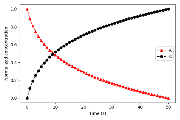
traj = solver.run()
ysim_array = traj.dataframe[obs_names].values
# normalize the values from 0-1 (see function definition below)
ysim_norm = normalize(ysim_array)

plt.figure(figsize=(6, 4))
if title is not None:
    plt.title(title)
plt.plot(t, ysim_norm[:, 0], '^r', linestyle='--', label='A')
plt.plot(t, ysim_norm[:, 1], 'ok', linestyle='--', label='C')
plt.ylabel('Normalized concentration')
plt.xlabel('Time (s)')
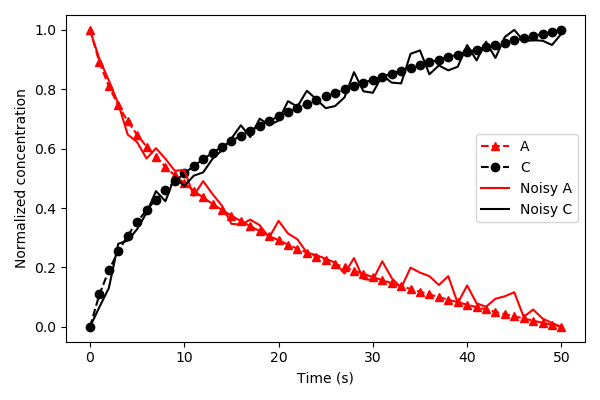
For training purposes, we will use the trajectories above and add some random noise.
noise = 0.05
noisy_data_A = norm_data[:, 0] + np.random.uniform(-1 * noise, noise, len(t))
norm_noisy_data_A = normalize(noisy_data_A)

noisy_data_C = norm_data[:, 1] + np.random.uniform(-noise, noise, len(t))
norm_noisy_data_C = normalize(noisy_data_C)

ydata_norm = np.column_stack((norm_noisy_data_A, norm_noisy_data_C))
plt.figure(figsize=(6, 4))
plt.plot(t, ysim_norm[:, 0], '^r', linestyle='--', label='A')
plt.plot(t, ysim_norm[:, 1], 'ok', linestyle='--', label='C')
plt.plot(t, norm_noisy_data_A, 'r-', label='Noisy A')
plt.plot(t, norm_noisy_data_C, 'k-', label='Noisy C')
plt.legend(loc=0)
plt.ylabel('Normalized concentration')
plt.xlabel('Time (s)')
Next, we define the cost function. The cost function should take a parameter set as an argument and return a scalar value, where the ultimate goal is to minimize this value. To efficiently sample across large parameter space, we use log10 space for the parameters. This means before you pass them back to the simulator, you must convert them to linear space. We are also only optimizing the rate parameters from the model, not the initial conditions, so we must create a mask to identify which parameters in the model are rate versus initial conditions. .. code-block:: python
rate_params = model.parameters_rules() rate_mask = np.array([p in rate_params for p in model.parameters]) param_values = np.array([p.value for p in model.parameters]) log_original_values = np.log10(param_values[rate_mask])
Here we use the chi square metric to determine the distances between the trajectory of the parameter sets and our training data.
def obj_function(params):
    # create copy of parameters
    params_tmp = np.copy(params)
    # convert back into regular base
    param_values[rate_mask] = 10 ** params_tmp
    traj = solver.run(param_values=param_values)
    ysim_array = traj.dataframe[obs_names].values
    ysim_norm = normalize(ysim_array)
    # chi^2 error
    err = np.sum((ydata_norm - ysim_norm) ** 2)
    # if there are nans, return a really large number
    if np.isnan(err):
        return 1000
    return err
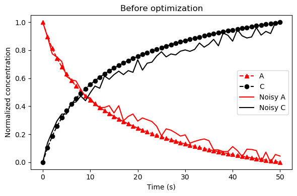
# make up a random starting point
start_position = log_original_values + \
                 np.random.uniform(-1, 1,
                                   size=len(log_original_values))
We can see that these are not ideal.
param_values[rate_mask] = 10 ** start_position
traj = solver.run(param_values=param_values)
ysim_array = traj.dataframe[obs_names].values
ysim_norm = normalize(ysim_array)

plt.figure(figsize=(6, 4))
plt.plot(t, ysim_norm[:, 0], '^r', linestyle='--', label='A')
plt.plot(t, ysim_norm[:, 1], 'ok', linestyle='--', label='C')
plt.plot(t, norm_noisy_data_A, 'r-', label='Noisy A')
plt.plot(t, norm_noisy_data_C, 'k-', label='Noisy C')
plt.legend(loc=0)
plt.ylabel('Normalized concentration')
plt.xlabel('Time (s)')
Finally, we get to initialize and run the PSO class. The main options to consider when running the algorithm are the num_particles, num_iterations, num_processors. The num_particles should be a multiple of the num_processors. You can set num_iterations as large as you’d like, but if you set it to a large value, you should consider setting the max_iter_no_improv or stop_threshold options.
# Here we initial the class
# We must provide the cost function and a starting value
optimizer = PSO(start=start_position, verbose=True, shrink_steps=False)

# We also must set bounds of the parameter space, and the speed PSO will
# travel (max speed in either direction)
optimizer.set_bounds(parameter_range=4)
optimizer.set_speed(speed_min=-.05, speed_max=.05)

# Now we run the pso algorithm
optimizer.run(num_particles=48, num_iterations=500, num_processors=12,
              cost_function=obj_function, max_iter_no_improv=25)
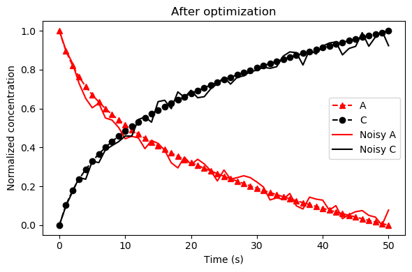
Done! We can then use optimizer.best.pos to access the best fit parameters.
best_params = optimizer.best.pos
param_values[rate_mask] = 10 ** best_params
traj = solver.run(param_values=param_values)
ysim_array = traj.dataframe[obs_names].values
ysim_norm = normalize(ysim_array)

plt.figure(figsize=(6, 4))
plt.plot(t, ysim_norm[:, 0], '^r', linestyle='--', label='A')
plt.plot(t, ysim_norm[:, 1], 'ok', linestyle='--', label='C')
plt.plot(t, norm_noisy_data_A, 'r-', label='Noisy A')
plt.plot(t, norm_noisy_data_C, 'k-', label='Noisy C')
plt.legend(loc=0)
plt.ylabel('Normalized concentration')
plt.xlabel('Time (s)')